Quantum Computation

Quantum computing is a way of carrying out computation using the laws of physics at the microscopic scale: the scale of individual atoms, individual photons, etc. Scientists have discovered that, for certain problems, computing in this way can be far more powerful than computing with the classical computers we use every day. An enormous scientific and technological effort is now under way to build quantum computers and realize this potential.

One of the key resources in quantum information science and quantum computing is entanglement. Entanglement describes correlations between separate quantum systems that have no equivalent in classical physics. It lies behind some of the strangest phenomena in quantum theory, from the Einstein–Podolsky–Rosen paradox¹ to quantum teleportation. And, in ways that are still not completely understood, entanglement appears to be intimately connected to the power of quantum computation.

Non-local quantum computation

Non-local quantum computation brings quantum computation and entanglement together in a very original way. The word non-local refers to the fact that the computation is distributed between parties that are physically separated. This raises many open questions and, hopefully, will provide deeper insight into both quantum computation and entanglement.

The basic problem is quite abstract. Imagine two parties, traditionally called Alice and Bob, who are in separate laboratories, or perhaps even separate cities. Alice has some quantum information and Bob has some quantum information, and they want to carry out a computation that depends on both of their inputs.

There is one important detail: their inputs are quantum information, not ordinary computer files. With ordinary files, they could each keep a copy, send a copy to the other, and do the calculation locally. An unknown quantum state cannot be copied in this way.²

There are several ways they might do this.

Let’s suppose the computation itself is very quick, so what takes time is sending the information from one place to another.

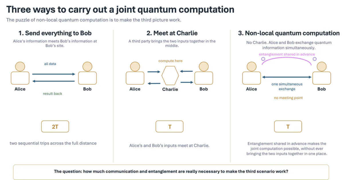
The simplest is for Alice to send all her information to Bob. Bob now has everything he needs to carry out the computation, after which he sends Alice whatever information she needs in return. If T is the time required for information to travel from Alice to Bob, this procedure takes a total time of approximately 2T: one trip there, followed by one trip back.

There is a more efficient possibility if we introduce a third party, Charlie, positioned exactly halfway between them. Alice and Bob can simultaneously send their information to Charlie. Charlie does the computation very quickly and then sends the results back to Alice and Bob. Since the information only has to travel half the distance in each direction, the entire process can be completed in time T.

In both cases, however, Alice’s and Bob’s information eventually meet somewhere. Their inputs are brought together so that they can interact.

Non-local quantum computation asks whether we can do something more surprising. Suppose there is no Charlie, and suppose the entire computation must still be completed in time T. Alice has time to send only one message to Bob, while Bob simultaneously sends one message to Alice. They cannot wait to receive a message and then respond: the two messages must cross each other in flight.

At first sight, it seems impossible that they could carry out a joint computation this way. Yet quantum mechanics provides another resource. If Alice and Bob share entanglement before the computation begins, then certain joint quantum computations can indeed be performed with only this single simultaneous round of communication.

This is the setting of non-local quantum computation.

The remarkable part is that, although such computations are possible, they are often extremely inefficient. Alice and Bob may need far more resources, in particular far more entanglement and communication, than would be needed if their quantum systems could simply be brought together. A fundamental question is therefore:

How much communication and entanglement are actually necessary to perform a given computation non-locally?

At first this can sound like a rather academic question. But non-local quantum computation has connections to several other areas of quantum information science, including cryptography, quantum simulation, and questions in quantum gravity related to the holographic principle. In its own small way, it is therefore a kind of “one problem to rule them all”. Progress on this problem may illuminate several apparently different questions at once.

Catalytic quantum computation

In the autumn of 2025, researchers from the Perimeter Institute for Theoretical Physics and the University of Waterloo in Canada and from the Université libre de Bruxelles in Belgium met at the Perimeter Institute to work on non-local quantum computation.

During their discussions they asked a deceptively simple question:

What happens to the entanglement after the computation is finished?

Entanglement is normally thought of as a resource that may be consumed during a quantum protocol. But the researchers realized that, for some computations, they could get the entanglement back at the end. It was needed to do the computation, but it was not used up.

That is quite fascinating: a resource that is required to do something, but that you still have afterwards. They call this catalytic entanglement. The word comes from chemistry, where a catalyst enables a reaction without being consumed by it.

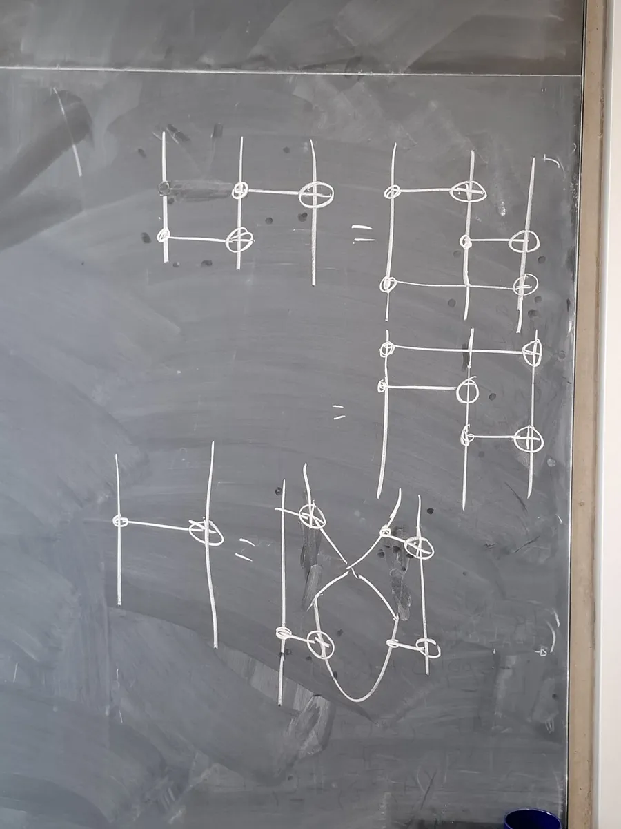
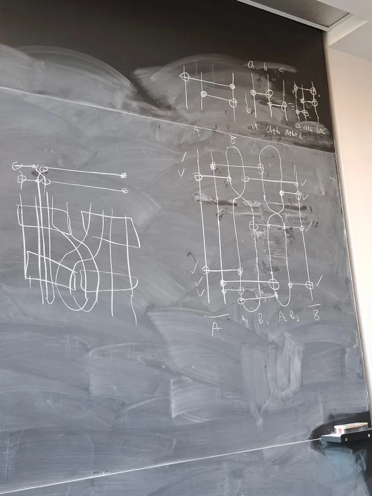
The researchers first found an example showing how a controlled-NOT gate, or CNOT, could be carried out in this catalytic non-local setting. When they met again the following week, they found a more complicated example involving a controlled-controlled-NOT gate, also known as a CCNOT or Toffoli gate.

From Science to Jewelry

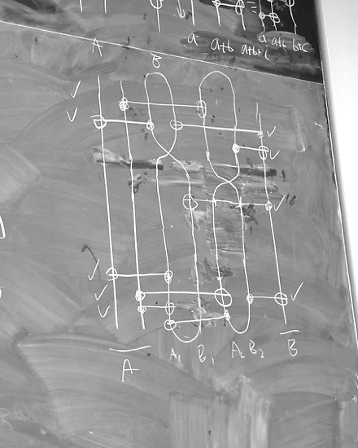
As they worked, they drew the quantum circuits on a blackboard. One of the researchers went to New York and the future founder of Studio Galois serendipitously saw the diagrams and decided to make jewelry depicting them. Some of those original brainstorming diagrams are shown below beside the Quantum Necklace they inspired.

Whether this idea will ultimately lead to a fundamental new insight into quantum computation and entanglement remains an open question. That uncertainty is itself part of the story.

Our quantum jewelry is therefore a picture of science in the making.

There is a small paradox here. The beauty of the jewelry does not depend on how profound the scientific result turns out to be. It only takes a beautiful diagram to inspire an artist.

Of course, we wish the scientists the best of luck, and hope that this work leads to many important results.

Appendix: Understanding Quantum Circuits and Quantum Computation

You do not need to understand quantum computing to appreciate the jewelry. But the lines and symbols are not arbitrary: they come from quantum circuit diagrams.

A circuit diagram is a way of showing what happens to qubits during a computation. Each line follows a qubit, and the symbols show the operations applied to it.

This appendix explains just enough of that language to read the pieces.

Bits and qubits

The basic unit of ordinary information is a bit. A bit has one of two possible values, conventionally written 0 or 1.

The physical representation does not matter. In an ordinary computer, a bit might correspond to the electrical state of a tiny component. Abstractly, it is simply something with two possible states.

A quantum computer uses quantum bits, or qubits. Their two basic states are normally written |0⟩ and |1⟩.

A qubit can be in either of these states, but quantum mechanics also allows something with no classical equivalent: a superposition of the two.

A qubit in superposition can be, for example, mostly |0⟩ and a little |1⟩. Measure it and you do not get a blurred in-between answer like 0.8: you get a plain 0 or a plain 1, at random, and from then on the qubit simply is what you found. If you prepare many qubits in that same state and measure them all, you will mostly get 0 and occasionally 1. This is not a statement about our ignorance: the qubit is not secretly 0 or 1 before we look. It really is in both states at once, in some proportions.

Superposition

A classical bit has a definite value: it is either 0 or 1.

A qubit can instead be in a superposition of |0⟩ and |1⟩. When we measure it, however, we still obtain an ordinary answer: either 0 or 1.

The power of superposition is subtler than saying that a quantum computer simply “tries every answer at the same time.” Quantum states have quantities called amplitudes,³ and amplitudes can reinforce or cancel one another through a phenomenon called interference.

A successful quantum algorithm is designed so that, as the computation proceeds, unwanted possibilities tend to cancel while useful ones are reinforced. Measurement can then reveal the desired result with high probability.

This interference is one of the essential ingredients of quantum computation.

Entanglement

With more than one qubit, something even stranger becomes possible.

Two quantum systems can share a state that cannot be described by assigning a separate state to each system individually. They are then said to be entangled.

For example, two qubits can be prepared so that, when they are measured, their results are always correlated, even when the qubits are far apart. A particularly important entangled state of two qubits is called a Bell pair, or an entanglement bit.

Entanglement does not allow Alice and Bob to send information instantaneously. But when it is combined with communication, it enables tasks that would otherwise be impossible or much more expensive. Non-local quantum computation is one example.

Quantum gates

A computation consists of operations performed on bits or qubits. Simple operations are called gates.

One familiar classical example is NOT. A NOT gate flips a bit: 0 becomes 1, and 1 becomes 0.

Quantum computation has its own collection of gates. The designs discussed on this page prominently feature two of them: the controlled-NOT and the controlled-controlled-NOT.

The controlled-NOT gate

The controlled-NOT, usually abbreviated CNOT, acts on two qubits. One is called the control and the other the target. The control qubit is left unchanged. If the control is |0⟩, nothing happens to the target. If the control is |1⟩, the target is flipped: |0⟩ becomes |1⟩, and |1⟩ becomes |0⟩.

In the standard circuit notation used by physicists, the control is represented by a dot and the target by a crossed circle, with a line joining the two.

The jewelry simplifies this graphical notation while preserving the structure of the circuit.

The controlled-controlled-NOT gate

The controlled-controlled-NOT, abbreviated CCNOT and also known as the Toffoli gate, extends the same idea to three qubits.

There are now two control qubits and one target. The target is flipped only when both controls are 1.

The addition of just one extra control turns the simple CNOT motif into a substantially richer circuit and, in the catalytic constructions that inspired these pieces, into a more elaborate visual form as well.

Shared entanglement and Bell pairs

In a non-local computation, Alice and Bob begin in different locations. Some of the qubits belong to Alice and others to Bob.

They may also begin with pairs of qubits that are already entangled. These shared Bell pairs are a resource prepared before the computation starts.

The central question is then how Alice and Bob can combine these shared entangled states with local quantum operations and a limited amount of communication to reproduce a computation that would normally require their quantum systems to meet.

How to read a quantum circuit

A quantum circuit is a diagram showing a computation unfolding through time. Physicists usually draw quantum circuits horizontally, with time flowing from left to right. In the jewelry, the circuit is rotated: time runs from bottom to top. Operations near the bottom occur earlier; operations higher in the design occur later.

Each line represents a qubit. Symbols placed along that line represent operations applied to it. When an operation acts on two or more qubits at once, its symbols are connected across the corresponding lines.

Bell pairs are represented by the paired structures at the beginning of the circuit.

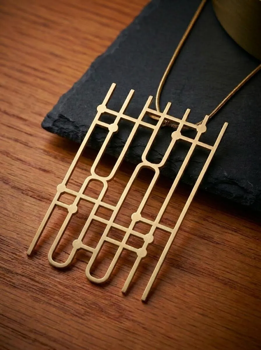
In the necklace version of the catalytic CCNOT construction there are seven qubit lines in total: two input qubits at Alice’s site, one input qubit at Bob’s site, and two Bell pairs (entangled bits) each represented by two qubit lines. The crossings in the design represent a real exchange of quantum information between Alice and Bob.

From a circuit to a piece of jewelry

The diagrams that inspired these pieces were never intended as drawings.

They were working scientific notation: lines, gates, crossings, and entangled states sketched on a blackboard as researchers tried to understand a new problem.

But quantum circuits already possess a visual grammar. Qubits become parallel lines. Gates connect them. Entanglement creates pairs. The movement and exchange of quantum information creates crossings, repetitions, and symmetries.

Seen outside their usual scientific context, those structures can look surprisingly architectural, or ornamental.

The jewelry preserves that connection to its origin. It is not merely inspired by quantum computing. Its geometry comes from actual quantum computations.

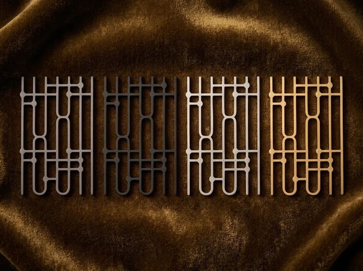
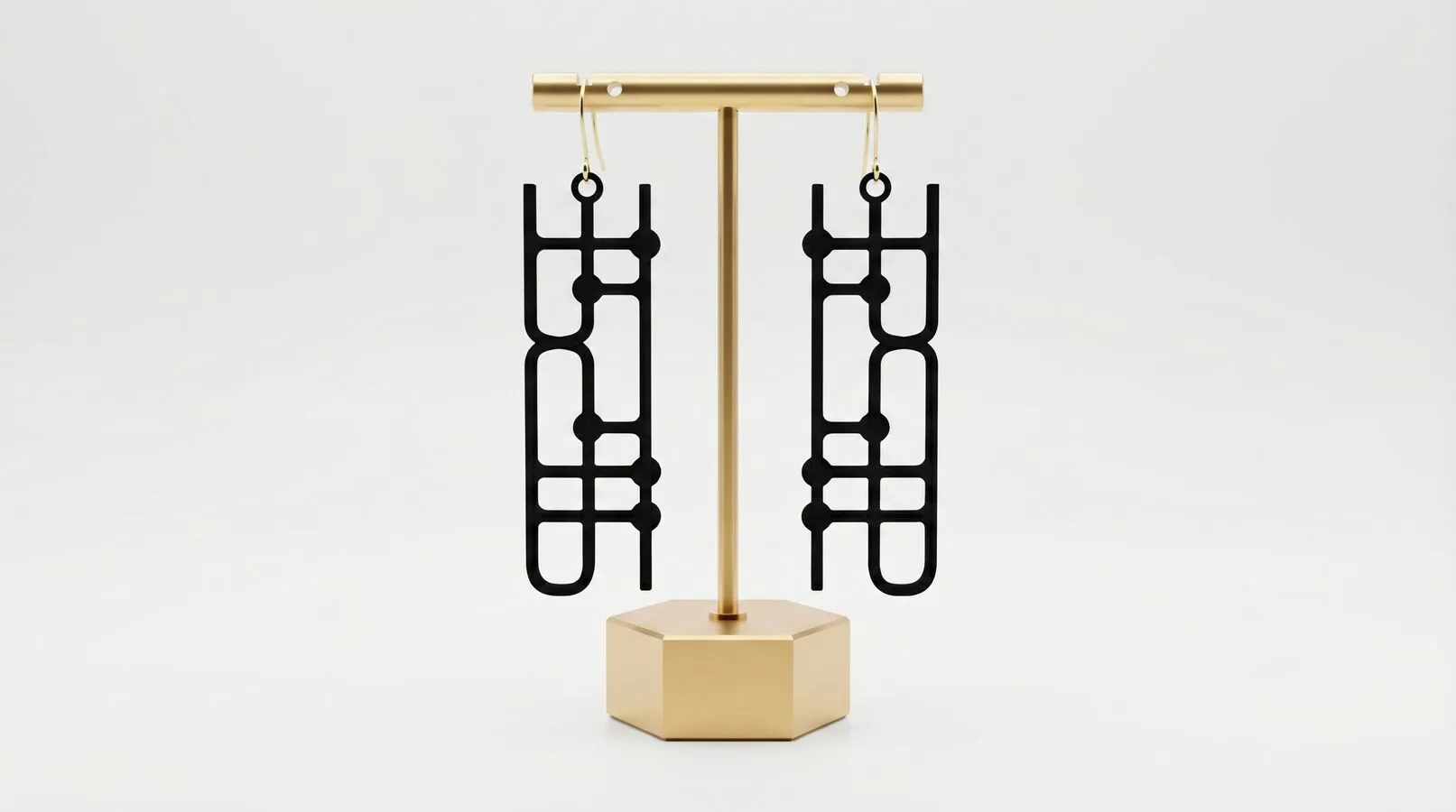
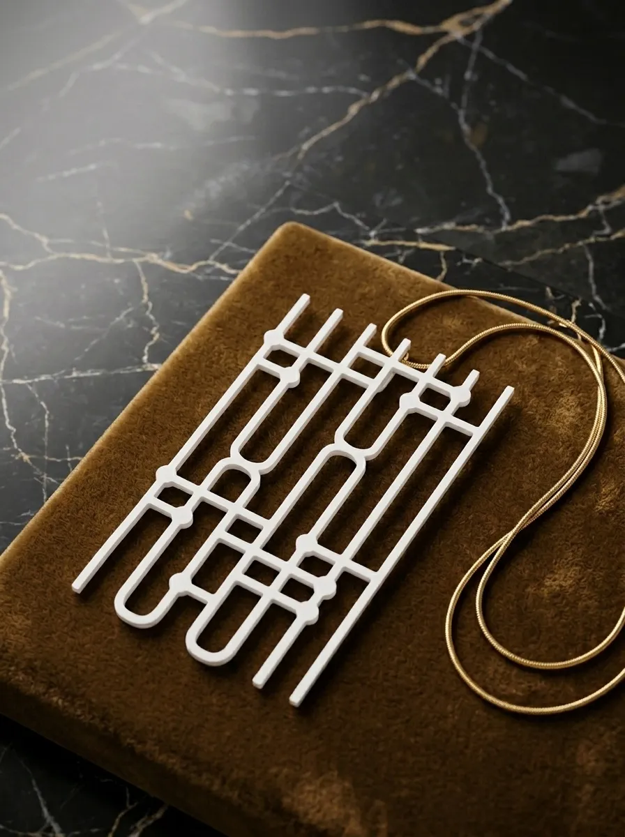
The necklace preserves the complete seven-line catalytic CCNOT construction in stylized form. The Earrings and Mini are deliberately smaller excerpts from the same circuit geometry rather than complete copies of the full protocol. A circuit of two or three qubits does not leave much to look at, so rather than invent a new, smaller circuit for the smaller pieces, we focused on a part of the necklace’s: each is a close-up of the full computation, adapted to its scale.

The result is both an object and a diagram: a small fragment of a scientific question, transformed into something that can be worn.

More Reading

Below are some references if you are interested in learning more about quantum computation.

• Quantum computing in a one page of comic. This covers about the same material as this page, in comic-book format. Don’t let the format fool you: it was done in collaboration with Scott Aaronson, who is both a computer scientist pushing the frontier of quantum computing and a first-class pedagogue.
• If you like videos. 3Blue1Brown (Grant Sanderson) is one of the premier mathematical pedagogues on YouTube. Here he covers quantum computation and explains Grover’s algorithm, a beautiful example of a quantum algorithm that seems to accomplish the impossible (impossible for a classical system that is).
• Quantum Computing Since Democritus. Freely available lecture notes by Scott Aaronson covering a wide range of topics. The notes are light on mathematics and physics but conceptually deep. The more you already know about the field, the more you will get out of them.
• Quantum Computation and Quantum Information by Michael A. Nielsen and Isaac L. Chuang. The standard master’s-level textbook. Best if you already have an undergraduate-level understanding of linear algebra and probability.

Notes

1. 1. In 1935 Albert Einstein, Boris Podolsky and Nathan Rosen published a famous thought experiment which they believed showed that quantum states must secretly have definite values that we simply do not know until we measure them (the alternative, which Einstein rejected, was “spooky action at a distance” between distant particles). It was not until 1964 that John Stewart Bell showed that no such “secretly definite” theory could reproduce the predictions of quantum mechanics, so we must accept that nature is genuinely bizarre. Many people thought that all this theory was very nice, but that if we actually did the experiments we would discover that nature is not that weird. The experiments were done, first by Stuart Freedman and John Clauser in 1972 and then decisively by Alain Aspect in 1982, and the theory was right all along. Aspect, Clauser and Anton Zeilinger shared the 2022 Nobel Prize in Physics for this work. So do not despair if you find all of this confusing: it has been a source of wonder and frustration for a very long time for very smart people.
2. 2. Quantum mechanics prevents duplication of state: given a qubit in an unknown state, it is impossible to make a copy of it, so Alice cannot keep her qubit and also send a copy to Bob so that both can inspect it and do things depending on that state. This is known as the “No Cloning Theorem”. While quantum computing makes some things much easier, some other things that are trivial in classical computing are impossible in quantum theory.
3. 3. Amplitudes are complex numbers. A qubit’s state is written α|0⟩ + β|1⟩, where α and β are complex numbers, and the probability of measuring 0 is |α|², the squared magnitude of the amplitude. So a qubit in the state (√3⁄2)|0⟩ + (1⁄2)|1⟩ gives a 3⁄4 chance of measuring 0 and a 1⁄4 chance of measuring 1. Because only the square is a probability, an amplitude is allowed to be negative, and so two contributions to the same outcome can cancel. Ordinary probabilities can never do this: adding chances only ever makes an outcome more likely.