
Computation
Computer science is not the study of computers. It is the study of what is computable, how, and how long it takes. But before you can even start studying this, you need to figure out what “computable” actually means.
This was figured out in the 1930s, before computers existed. The best known answer is Alan Turing’s machine. It is in that framework that many theoretical results of computer science are usually explained, like the halting problem.
Before Turing there was already another, equivalent, model of computation, which is the one used in our jewelry: lambda calculus, invented by Alonzo Church. Lambda calculus is maybe less well known than Turing Machines, but it had, and still has, a huge impact on computer science, programming and programming languages.
Lambda calculus
Lambda calculus only knows about functions, nothing else: no names, no numbers, nothing but functions.
In regular math you define a function by writing something like f(x) = 3x + 4. The customary notation in lambda calculus, and the one we will use here, is λx. 3x + 4: the Greek letter lambda indicates you are defining a function, the dot plays the same role as the equals sign in the regular notation, and then comes the body of the function. The body is what the function returns when you apply it to something. When you apply the function, like f(7), you write the function next to its argument: (λx. 3x + 4) 7.
You may wonder what 3, 4 and 7 are here, since lambda calculus only has functions, and what is the “plus” and the “multiply”. For numbers we identify specific functions as representing them: a function that does something four times is the number 4. The + and the × are functions too.
To apply a function, you take its body, and each time the variable appears you replace it by the argument. For most expressions you will have to do that many times until there is nothing left to replace, and what remains is the answer.
Lambda diagrams
Making jewelry out of this notation would be very difficult. Luckily, John Tromp invented a way to represent lambda expressions as diagrams. Those diagrams are our jewelry.
Going from an expression to a diagram is easy.
- For every λ you draw a horizontal line.
- For every x that appears in the body, you draw a vertical line hanging from that horizontal line.
- When a function is applied to an argument, you join the two by a link at the bottom, the function on the left and the argument on the right.
Here is the number two, the function that takes f and x and does f twice: λf. λx. f (f x). From here on we write λf x. as a shorthand for λf. λx..
Applying a function can be seen as an expression being rewritten, or as a diagram modifying itself. Below, λx. x x is applied to λy. y.
The Recursion Earrings
Recursion is the idea that a function calls itself. For example, the factorial is generally defined as:
factorial(0)  =  1
factorial(n)  =  n × factorial(n − 1)
Note that the function appears on both sides of the equals sign: it is recursive.
This seems impossible to do in lambda calculus, because we don’t have names for functions. Where the definition says factorial, you would have to write out the whole function instead. And inside that copy, write it out again. You would never finish.
Luckily, there is an extremely elegant idea that lets you do it anyway. You can find an expression which takes a function and hands it to itself. It is called the Y combinator:
λf. (λx. x x) (λx. f (x x))
To use it, add an argument to the function and use that argument whenever you want to do a recursive call. For example, factorial becomes factorial(r, n) = n × r(n − 1). When you give this function to the Y combinator, it will supply the function itself in that new r argument. A very simple example to illustrate this is a function that counts to infinity:
toInfinity(n) = toInfinity(n + 1)
With the new argument r it becomes λr n. r (n + 1). Here is the full expression, started at one, with its diagram and what happens when it runs:
(λf. (λx. x x) (λx. f (x x))) (λr n. r (λf x. f (n f x))) (λf x. f x)
1 the Y combinator 2 toInfinity 3 n + 1 4 one
In the animation above, you see the number in the upper right-hand corner getting bigger and bigger: 1, 2, 3.
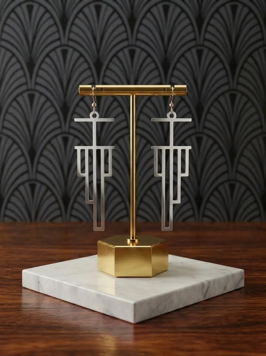
The Recursion Earrings are the Y combinator, that magical expression that allows recursion in a setting where you cannot name things.
λf. (λx. x x) (λx. f (x x))
=
Graham’s Necklace
Graham’s number is a mind-bogglingly huge number. It became famous in 1977, when Martin Gardner wrote in Scientific American that it was the largest number ever used in a serious mathematical proof.
To explain how big it is, we need a little notation.
Multiplication is to addition what exponentiation is to multiplication. What we mean by this is that multiplication is repeated addition: 5 × 3 = 5 + 5 + 5. In the same way, exponentiation is repeated multiplication: 5³ = 5 × 5 × 5. We can repeat this idea and define an operation, called tetration, which is repeated exponentiation, and then define an operation that is repeated tetration, and so on as long as we like.
The standard notation for this is Knuth’s up-arrows. One arrow is the power: 5 ↑ 3 is 5³. Two arrows is repeated exponentiation, three arrows is repeated two-arrows, and so on.
| multiplication | 5 × 3 | 5 + 5 + 5 |
| power | 5 ↑ 3 | 5 × 5 × 5 |
| tetration | 5 ↑↑ 3 | 5 ↑ 5 ↑ 5 |
| and again | 5 ↑↑↑ 3 | 5 ↑↑ 5 ↑↑ 5 |
| and so on | ⋮ | ⋮ |
As the number of arrows grows, the results get bigger at an incredible rate. 3 ↑↑ 3 is already 7,625,597,484,987, and 3 ↑↑↑ 3 is a tower of threes that many levels high.
Graham’s number is defined in a way where the number of arrows itself grows faster and faster. Start with 3 ↑↑↑↑ 3, four arrows, and call it g₁. Then g₂ is 3 and 3 with g₁ arrows between them, g₃ is the same with g₂ arrows, and so on. Graham’s number is g₆₄.
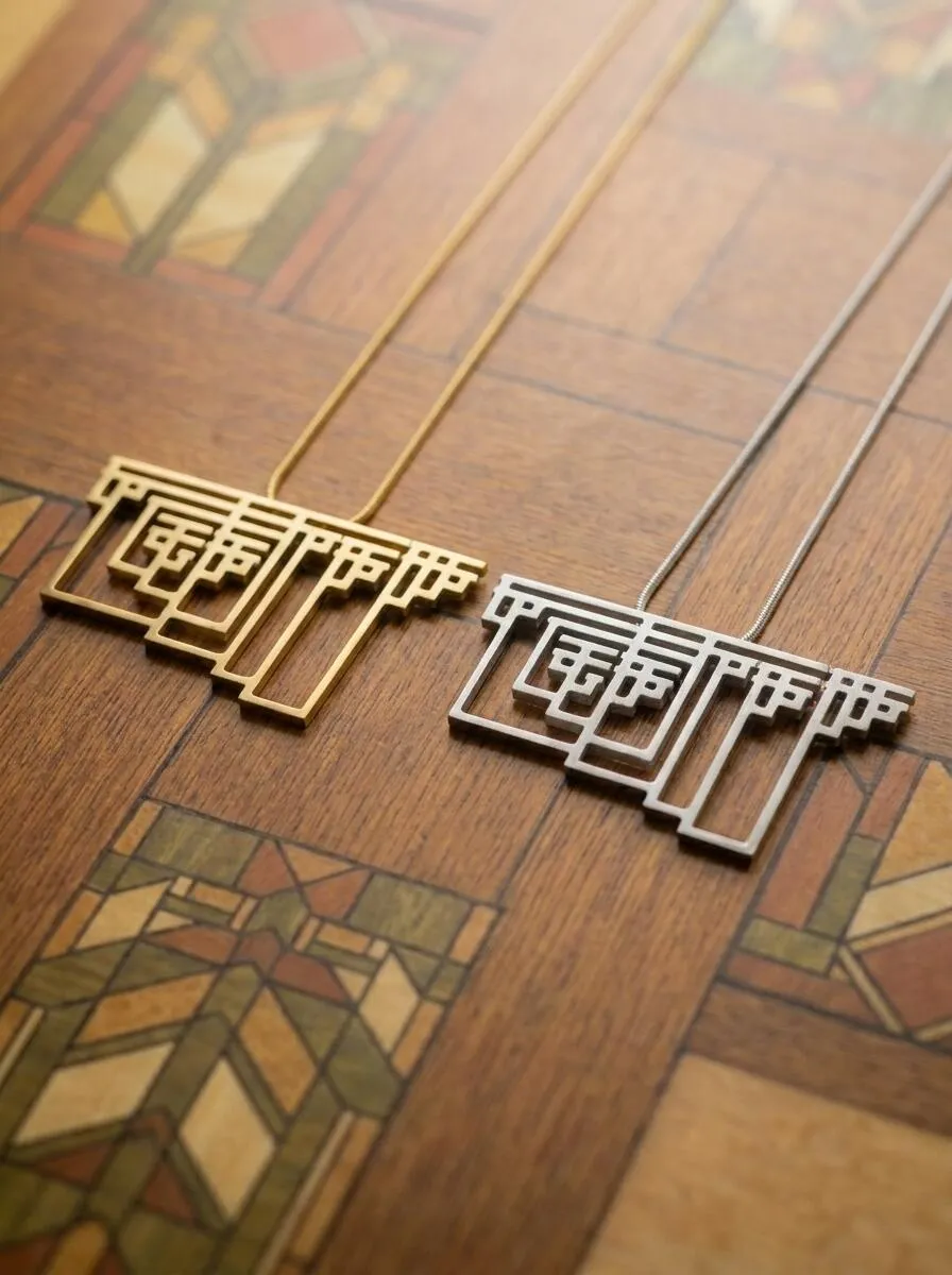
This number is stupendously big. It cannot be written down in this universe with any usual notation, but we can find quite small programs that compute it, and one such program is Graham’s Necklace.1

(λc3. (λc2. c3 (c2 c2) (λn. n (λf b. b f (λx. x)) (λb f. c3 (b f)) c3) (c2 c2))
(λf x. f (f x)))
(λf x. f (f (f x)))
| 1 | λf x. f (f x) | the number two: the value given to c2 |
| 2 | λf x. f (f (f x)) | the number three: the value given to c3 |
| 3 | c2 c2 | four: 2 applied to 2 is 2² |
| 4 | c3 (c2 c2) | sixty-four: 3 applied to 4 is 4³ |
| 5 | λb f. c3 (b f) | multiply by three |
| 6 | λf b. b f (λx. x) | the next operation up |
| 7 | λn. n (6) (5) c3 | one round: 3, n arrows, 3 |
The second and third lines of the expression are numbers we have already seen: λf x. f (f x) is two and λf x. f (f (f x)) is three. The first line is a function of two variables, c3 and c2, which are just names, like x or y. The whole expression applies that function to the two numbers.
The two and the three on the right, parts 1 and 2, are the only numbers drawn in full. The whole of Graham’s number is computed from them.
We can write the program, but trying to animate it would face a few difficulties. Before the animation finishes the diagram would become huge, your computer would run out of memory, the sun would become a red giant and swallow the earth, the universe would reach heat death. Everything is small before Graham’s number.2

More Reading
Below are some references if you are interested in learning more about the lambda calculus, lambda diagrams, and Graham’s number.
- A Tutorial Introduction to the Lambda Calculus. A short, readable introduction for anyone who wants to really understand lambda calculus.
- The Little Schemer, by Daniel Friedman and Matthias Felleisen. A thorough introduction to recursion and the Y combinator, in the style of a Socratic dialogue, through the Scheme programming language.
- Lambda Diagrams. John Tromp’s page introducing lambda diagrams.
- How to draw lambda diagrams. A tutorial with many worked examples, for anyone who wants to draw their own.
- Lambda calculus and Graham’s number and A picture of Graham’s number. Paul Crowley’s posts constructing the Graham lambda expression.
- Lambda Diagrams in motion. Paul Brauner’s animations of lambda diagrams computing.
- What is PLUS times PLUS? If you like videos: a beautifully animated introduction to the lambda calculus and lambda diagrams, by 2swap.
- Graham’s Number. Tim Urban’s long, funny attempt to convey how big it is.
Notes
- 1. The specific program was found by Paul Crowley, who has been making it shorter since 2012 on his blog Minds aren’t magic.
- 2. To pure mathematicians this might not be true: they don’t think of numbers as big or small. Graham’s number is but a tiny speck compared to infinity. And much bigger numbers have since appeared in serious mathematical literature.